Outstanding jobs per customer, engineer or job type
With Okappy, you can generate reports to see the outstanding jobs per customer, employee or subcontractor or the outstanding jobs by job type.
There are a couple of ways you can do this, read on to find out more.
To view outstanding jobs by customer, employee and job type on the job dashboard
- Click the filter
- Select Outstanding jobs
- Type in the customer name, job type and engineer’s name in the filter box
Download a short video to see how it’s done. Download video
To view outstanding jobs by customer, employee and job type as a report
- Go to the Reports screen

- Click Jobs and then select All jobs
- Enter a date range covering the period when the jobs were added
- Select Date added in the dates type drop down
- Click Generate report

You can then use the filter to quickly see the job done by customer, job type or name of the engineer or subcontractor that the job was assigned to.

To create a dashboard in Google Sheets using data from Okappy,
- Click the Google Sheets icon above the report
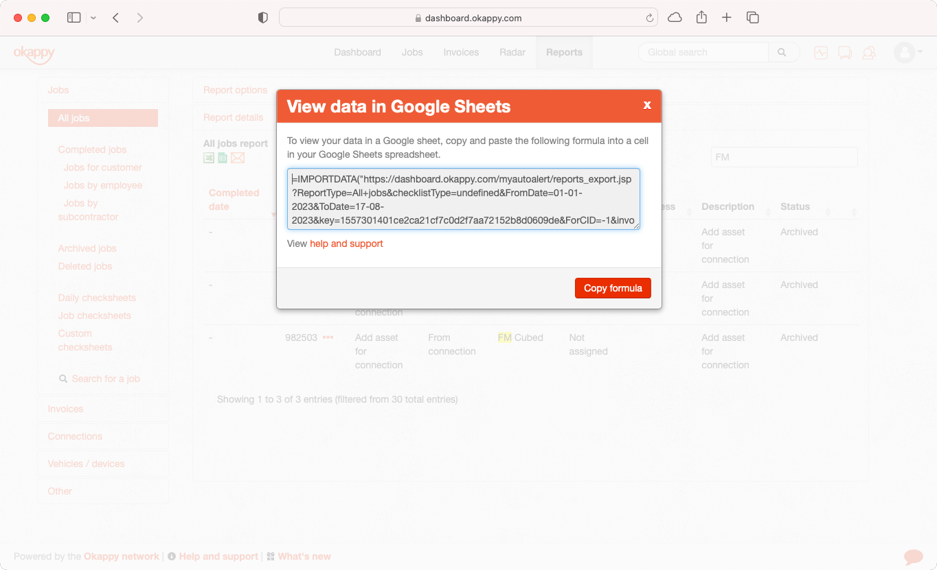
- Click Copy formula
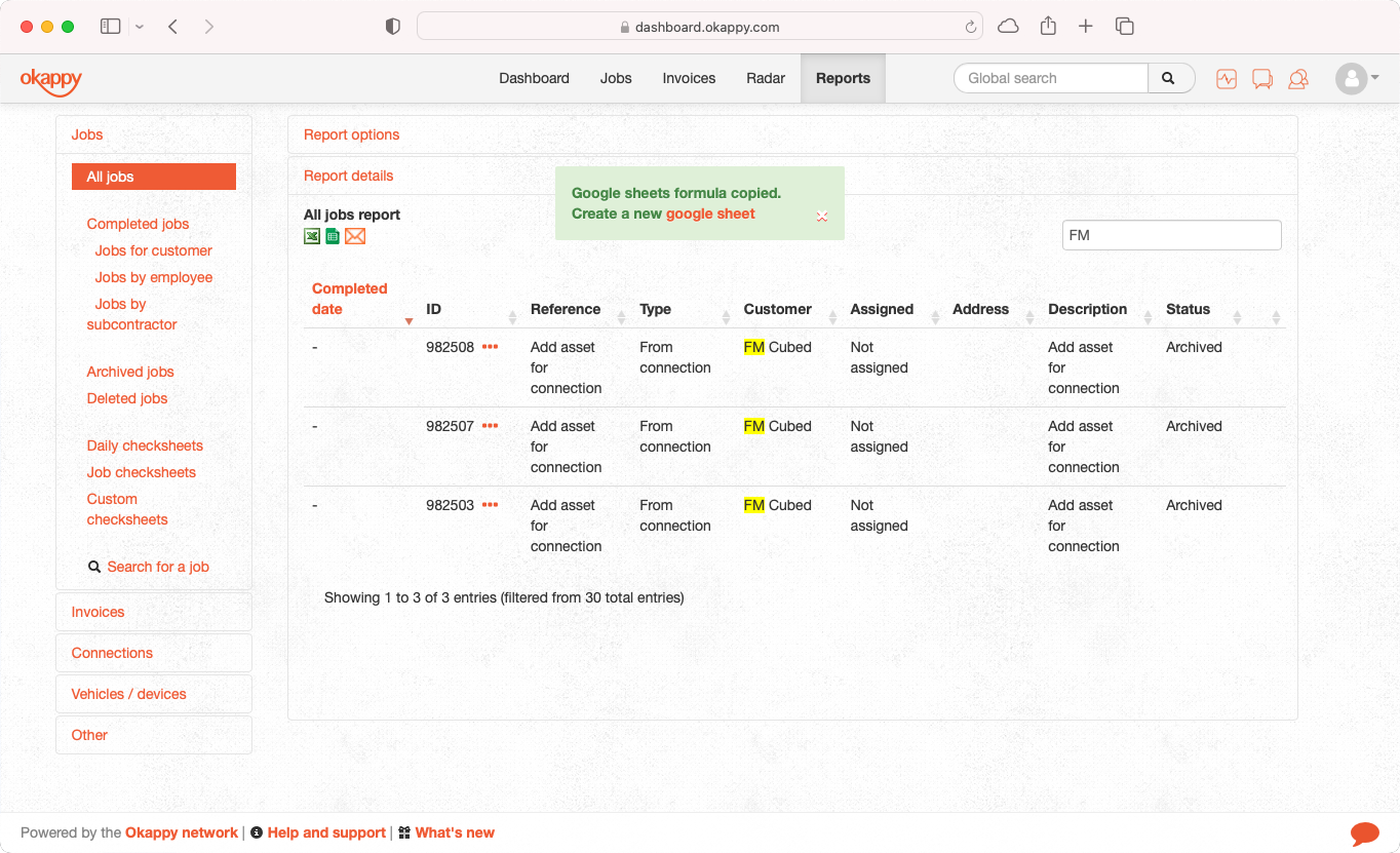
- Click Create a new sheet in the alert which pops up (or create a google sheet by typing sheets.new in the address bar, or from within Google sheets)
- In the new Google sheets, select a cell and paste the copied formula
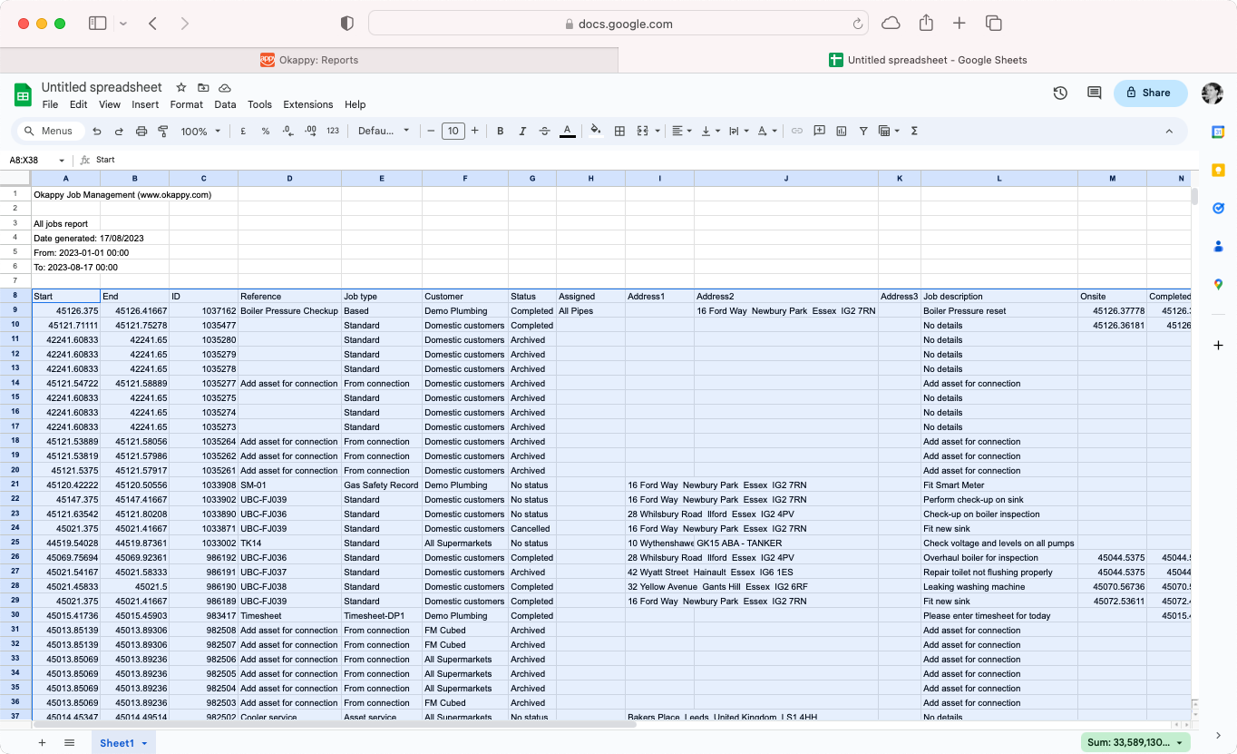
- Highlight the cells containing all the data which has been pulled down from Okappy
- At this stage, you may want to change column widths and change the types of different cells
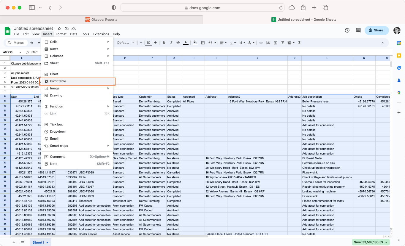
- Click Insert from the Google Sheets menu
- Select Pivot table
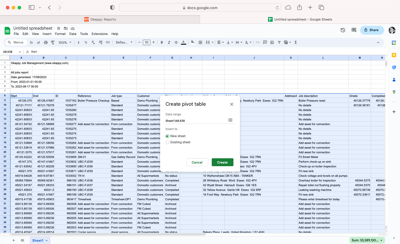
- Select New sheet
- And then click Create
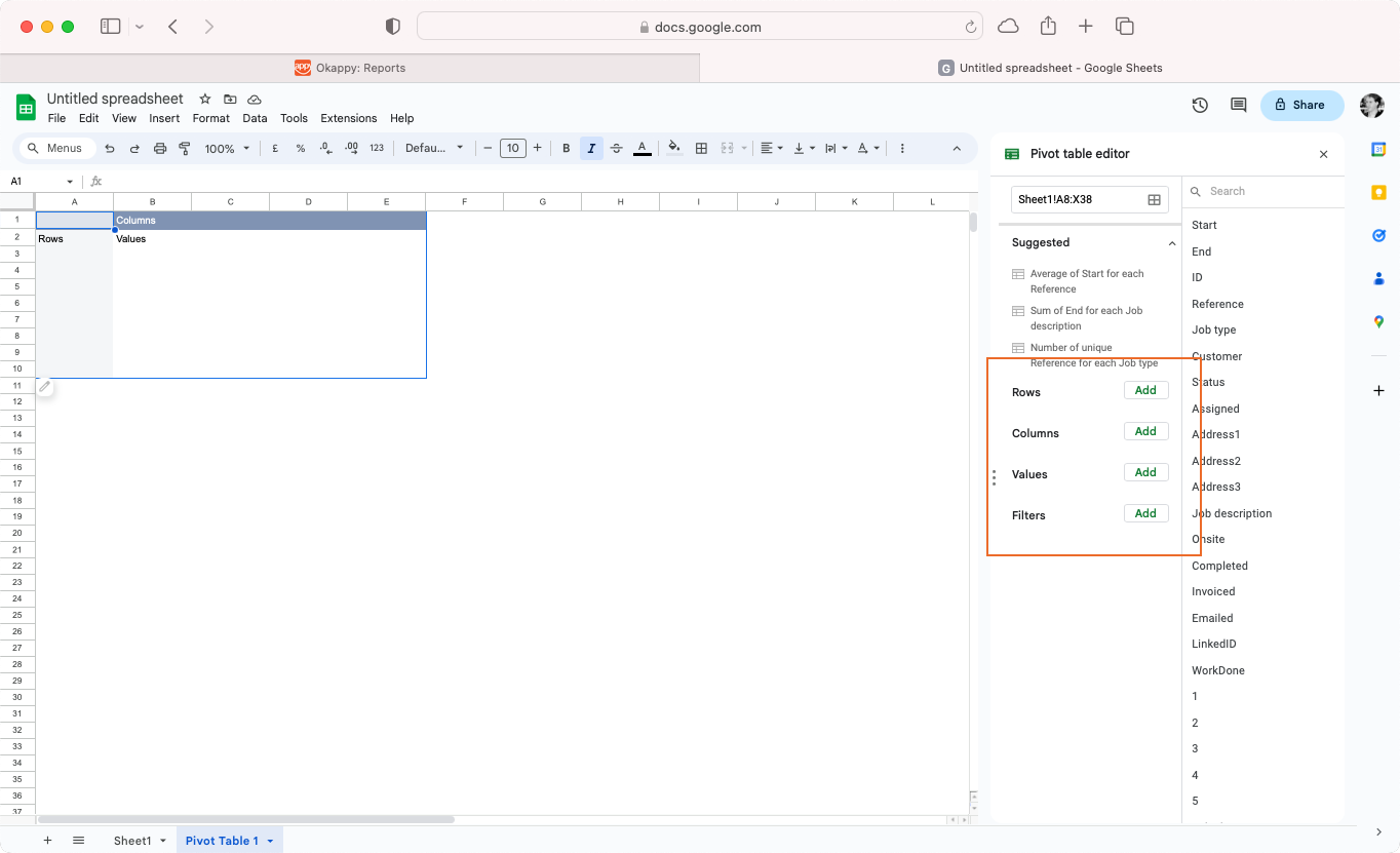
- Click a cell in the pivot table and then select the following options in the Pivot table editor section on the right of the sheet
- Click Add in the Rows section
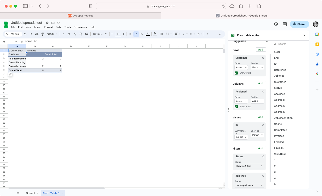
- Select Customers
- Click Add in the Columns section
- Select Assigned
- Click Add in the Values section
- Select ID and then select Count in the Summarise by option
- Click Add in the Filters section
- Select Status and select the following statuses: No status, On site and Work done
- Click Add in the Filters section again
- Select Job type
- Select the relevant job type you want to see the data for
To have Google Sheets update the pivot table automatically.
- Go to the tab which contains the original downloaded data
- Select the cell where you originally pasted the formula from Okappy
- Find the part of the formula which contains ToDate
=IMPORTDATA(“https://www.okappy.com/myautoalert/reports_export.jsp?ReportType=All+jobs&FromDate=01-01-2019+09:00&ToDate=29-08-2019+17:00&key=15569099553381b50cfe22c0a3167e174cef4dccd8&ForCID=-1&invoiceType=raised&UserID=2&description=-1″)
- Replace the data and time with &TEXT(TODAY(), “mm-dd-yyyy 23:59”)
=IMPORTDATA(“https://www.okappy.com/myautoalert/reports_export.jsp?ReportType=All+jobs&FromDate=01-01-2019+09:00&ToDate=”&TEXT(TODAY(), “mm-dd-yyyy 23:59″)&”&key=15569099553381b50cfe22c0a3167e174cef4dccd8&ForCID=-1&invoiceType=raised&UserID=2&description=-1″)
Further information
For further information about the reports you can generate from within Okappy, check the reports section of our support site. Alternatively, check out the questions and answers in our forum.